qscat
Validated quantum-scattering numerics for electron–diatomic collisions
A CPU-first Python library for electron–molecule scattering on finite-element DVR grids with exterior complex scaling. It computes the exact result and the approximations of the same quantity from one model definition — which is what makes an approximation testable rather than merely usable.
What this is
The method is not new: it is Rescigno and McCurdy’s FEM-DVR-ECS applied to Houfek, Rescigno and McCurdy’s two-dimensional resonant-collision model. What appears to be new is that it is released as a library. As of a survey on 2026-08-16, no released implementation was found of the two-dimensional resonant electron–diatomic model as a library, of an automatic FEM-DVR-ECS discretisation tuner, or of a complex-symmetric MUMPS backend with symbolic-analysis reuse across an energy sweep. That is a statement about the public record on the survey date, not about what exists.
The research stance decides the design: the exact solution is the oracle, and the approximation is what is under test. The library computes both from one model definition, on the same grids, so the difference between them is the measurement.
The model potentials are testbeds for finding where approximations fail, not descriptions of real molecules. Nothing here is fitted to or compared with experiment, and agreement with a published calculation certifies that the solver correctly solves that model — not that the model is physically realistic. N₂ is the only molecule with independent external data; for NO, F₂ and O₂ the exact solver is itself the reference, so agreement there is self-consistency between two routes through one repository.
Methods
Each one is checked against an analytic benchmark, a conservation law, a convergence study, or an independent reference implementation before it ships.
Exact two-dimensional driven solver
A driven Lippmann–Schwinger solve on the full electronic × nuclear grid, with no local reduction and no separation of the two coordinates. This is the oracle everything else is measured against.
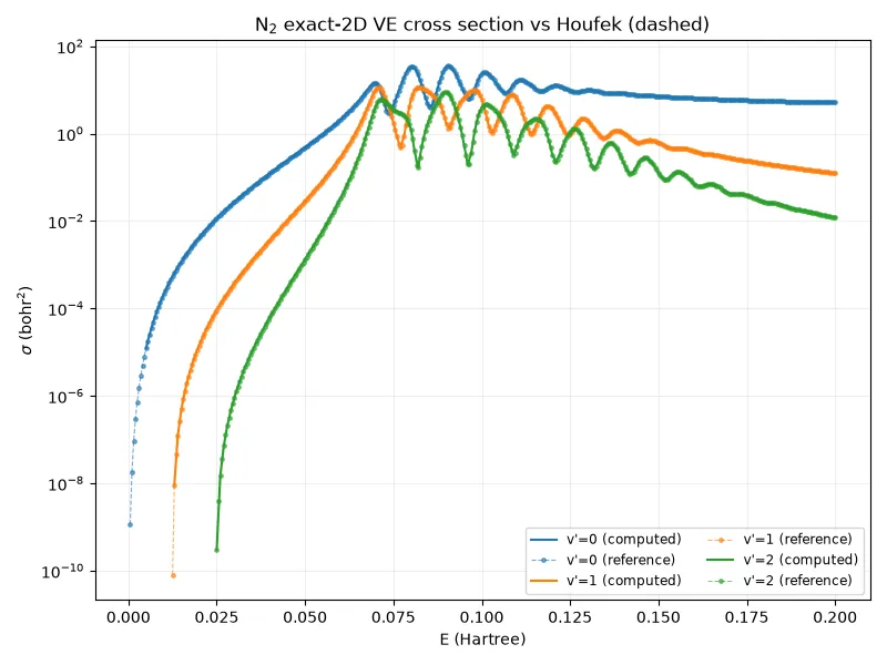
Measured: Reproduces published N₂ cross sections to 1 part in 10⁶ at the tightest anchor
Time-dependent wavepacket route
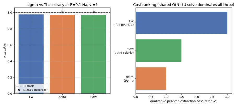
An order-3 diagonal-Padé propagation of an incident wavepacket, with three interchangeable energy extractors reading the same stored trajectory.
Measured: 161 energies from one propagation; median ratio 0.9984 against the time-independent result
Nonlocal resonance model
The rung between the local approximation and the exact solve: a complex, energy-dependent kernel that keeps the nonlocality a local complex potential throws away. Time-independent and time-dependent halves, each validated against the other.
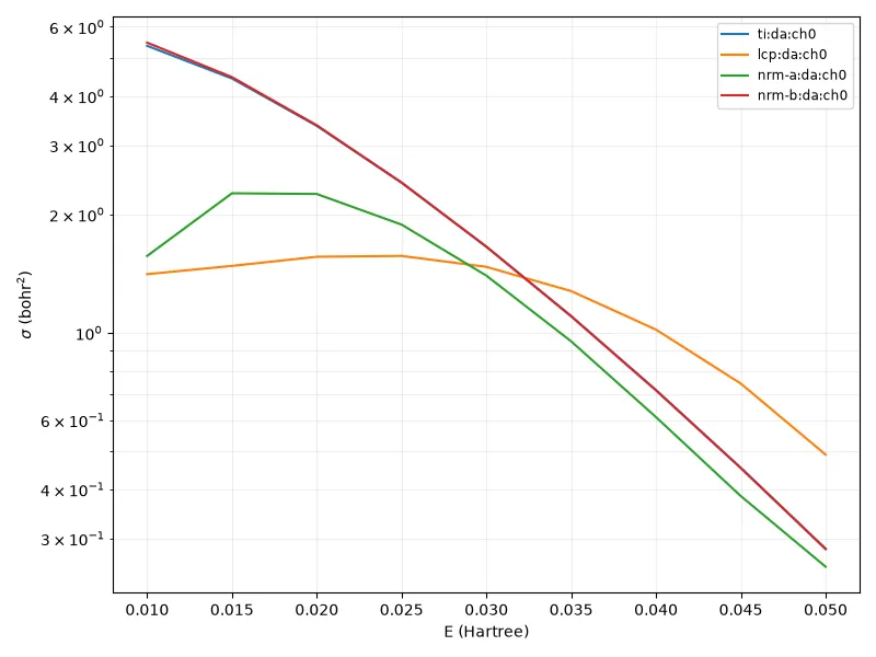
Measured: Within 0.06–1.9% of the exact oracle on F₂ dissociative attachment
Local complex potential
The standard approximation, implemented alongside the exact result rather than instead of it — which is what makes it testable rather than merely usable.
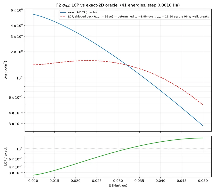
Measured: Error is systematic and energy-dependent: 0.263 → 1.736 across one F₂ sweep
Resonance states, approximate and exact
Quasi-bound levels in the Born-Oppenheimer picture, and the poles of the full two-dimensional S-matrix found by requiring stability under two independent exterior-scaling angles — plus the overlap test that decides whether a pole is a resonance at all.
Measured: On H₂⁺, four of 57 angle-stable poles were shown not to be resonances
Discretisation tuner
Derives a finite-element DVR grid from the potential and the energy range instead of hand-tuning element lengths. Grid parameters in this field are normally published as hand-tuned tables.
Measured: Converges F₂’s σ_DA on its first a-priori pass, at 1.027× the size of an expert hand-tuned deck
Potential factory
Fits model surfaces to target curves, so a new molecule is a fitted potential plus validation rather than new solver code.
Measured: Round-trips three published models’ own curves to 1e-3–1e-4 relative
Complex-symmetric sparse backend
A MUMPS SYM=2 factorization behind a solver-agnostic API, with symbolic-analysis reuse across an energy sweep and SuperLU kept as both fallback and differential oracle.
Measured: 81.3× faster factorization and 11.9× smaller peak memory at 143k unknowns
Findings
Measured results, each with the limit that travels with it. Nothing here is compared with experiment.
The exact two-dimensional solver reproduces an independent published calculation
Agreement to 1 part in 10⁶ at the tightest anchor, gated at rtol = 1e-3 against Karel Houfek’s CSVE.V00.J00 data
This certifies that the solver correctly solves that model — not that the model is a physically realistic N₂. No model parameter was tuned to improve agreement with anything.
The nonlocal resonance model recovers what the local approximation discards
F₂ dissociative attachment within 0.06–1.9% of the exact oracle where the local-complex-potential method is off by 11–74%; vibrational excitation better than 0.7% on N₂ and F₂
A differential comparison — both routes run on the same grids — so it validates the model reduction, not the grid. For F₂ this is self-consistency between two routes through one repository; only N₂ has independent external data.
The local approximation’s error is systematic and energy-dependent, not a fixed percentage
On F₂ the ratio to the exact result sweeps 0.263 → 1.736 across 0.010–0.050 Ha, crossing unity near 0.032 Ha — under-predicting below, over-predicting above
Measured on F₂, where the exact two-dimensional solver is itself the oracle: agreement elsewhere in this comparison is self-consistency between two routes through one repository.
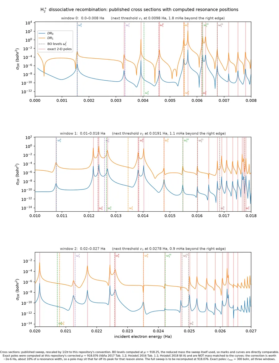
Exact non-Born-Oppenheimer poles land on published peak positions where the approximation drifts
H₂⁺ poles sit within 0.2–0.3 resonance widths of the published σ_DR peaks across three energy windows; the Born-Oppenheimer levels degrade 0.8 → 3.7 → 30.4 widths
Angle stability is necessary and not sufficient: four of 57 poles were not resonances at all, and 18 more are box-limited and are excluded from every number here.
A complex-symmetric direct solver puts a full energy sweep inside an hour
MUMPS SYM=2 against SuperLU on the 143k-unknown production deck: 81.3× faster factorization (3.2 s vs 258 s) and 11.9× smaller peak memory (0.6 GB vs 7.4 GB)
Residuals agree across backends to ~1e-12 — the two engines compute the same solution, only the cost differs. SuperLU remains the fallback and the differential oracle.
Three independent instruments pointed at one trajectory agree
Tannor–Weeks, Dirac and Flux extractors driven by a single N₂ propagation land within 0.6–0.7% of each other and 2.3–3.0% of the time-independent oracle
Their spread is a convergence diagnostic rather than a disagreement: it shrinks from ~20% on a reduced grid to ~3% as the grid and propagation length converge.
Wavefunctions
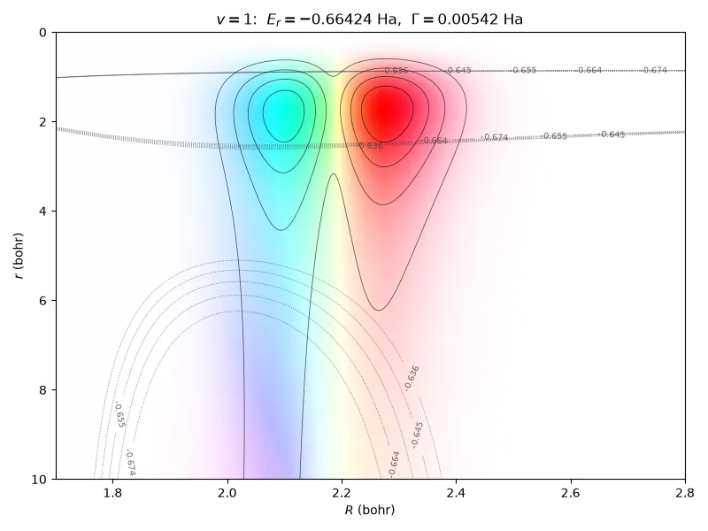
R horizontal, r vertical increasing downward, complex phase as hue, magnitude as brightness, potential contours in grey. Brightness is one global scale per panel; relative phase across a panel is meaningful, absolute hue is not.
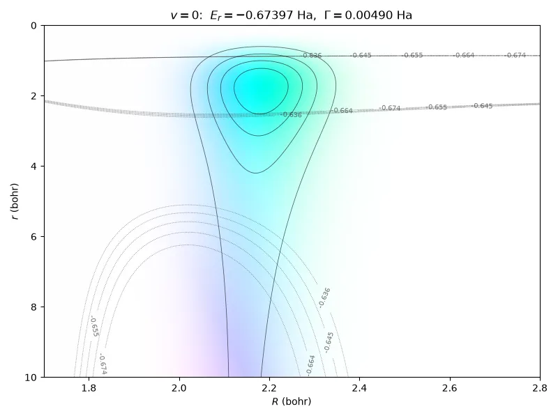
N₂⁻, v = 0: a single lobe of the trapped electron at r ≈ 1–3, R ≈ 2.2. The core is nearly real and the tail saturates at the travelling-wave value — the state is quasi-bound where it is bright and purely outgoing where it is faint, which is what a resonance is. N₂⁻, v = 1: the expected nuclear node, visible both as two lobes in R and as the phase flip across them. 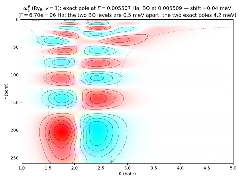
ω₁⁹ (Ry₉, v = 1): diffuse, about nine radial lobes reaching past 250 bohr, one node in R. Overlap with its Born-Oppenheimer product 0.970 — nearly pure, and it barely moves. 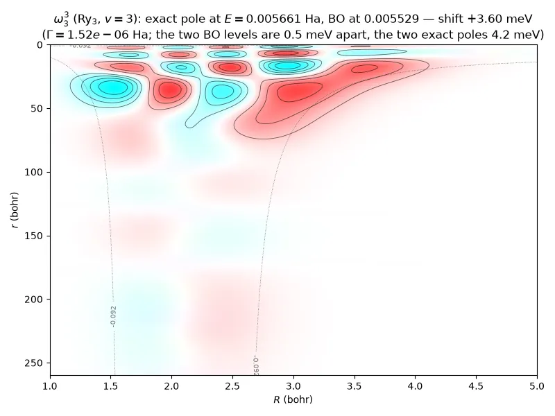
ω₃³ (Ry₃, v = 3): compact, confined inside about 70 bohr, three nodes in R. Overlap 0.783 — strongly mixed, and it carries almost the whole 4.2 meV splitting of this near-degenerate pair. 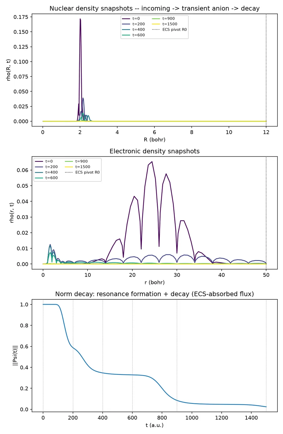
Formation and decay of the transient anion. The nuclear density starts sharply peaked near the N₂ equilibrium bond length and collapses as the resonance depletes; the electronic density shows the incoming wavepacket’s interference lobes collapsing toward zero. The lower panel is the norm decay, with the snapshot times marked.
Get started
qscat is not published to PyPI, and will not be until the citation article is out. Install it from the repository:
git clone https://github.com/VanaMartin/qscat
cd qscat
uv sync --all-packages
A first cross section, in twelve lines:
import numpy as np
from qscat.core import ScatteringProblem
from qscat.core.grids import electronic_grid, nuclear_grid
from qscat.dvr import TensorGrid
from qscat.model import N2

grid = TensorGrid([
    electronic_grid(r_max=16.0, order=7, n_complex=5),
    nuclear_grid(r_max=22.0, quadrature=10, n_complex=5),
])
prob = ScatteringProblem(grid=grid, model=N2, n_vib=4, v_init=0)

sigma = prob.ve_cross_section(vprimes=[0, 1, 2], E=np.array([0.10, 0.15, 0.20]))
print(sigma)  # (3, 3) bohr², [E, v']
Or drive it from configuration. One YAML file puts the exact oracle and the approximations on one axis — methods: [ti, lcp, nrm] — and writes cross sections, plots and a reproducibility manifest:
uv run qscat-run run apps/qscat-run/examples/n2-ve.yaml --output runs/n2-veEverything is in atomic units. The full API reference is in the documentation.
Citing qscat
If you use qscat directly in research, citation is required. Cite the software itself and the published work it implements. There is no software DOI and no method paper yet; the repository carries a CITATION.cff.
- , Time-dependent formulation of the two-dimensional model of resonant electron collisions with diatomic molecules and interpretation of the vibrational excitation cross sections, Phys. Rev. A 95, 022714 (2017). doi:10.1103/PhysRevA.95.022714
- , A model of resonant collisions of electrons with molecules and molecular ions, Doctoral thesis, Charles University, Prague, 2017. https://dspace.cuni.cz/handle/20.500.11956/92902
- , Numerically solvable model for resonant collisions of electrons with diatomic molecules, Phys. Rev. A 73, 032721 (2006). doi:10.1103/PhysRevA.73.032721
- , Numerical grid methods for quantum-mechanical scattering problems, Phys. Rev. A 62, 032706 (2000)
Released under the BSD 3-Clause licence.
Feedback and suggestions
Questions about the methods, a molecule you would like modelled, or a problem with the numbers — all welcome.